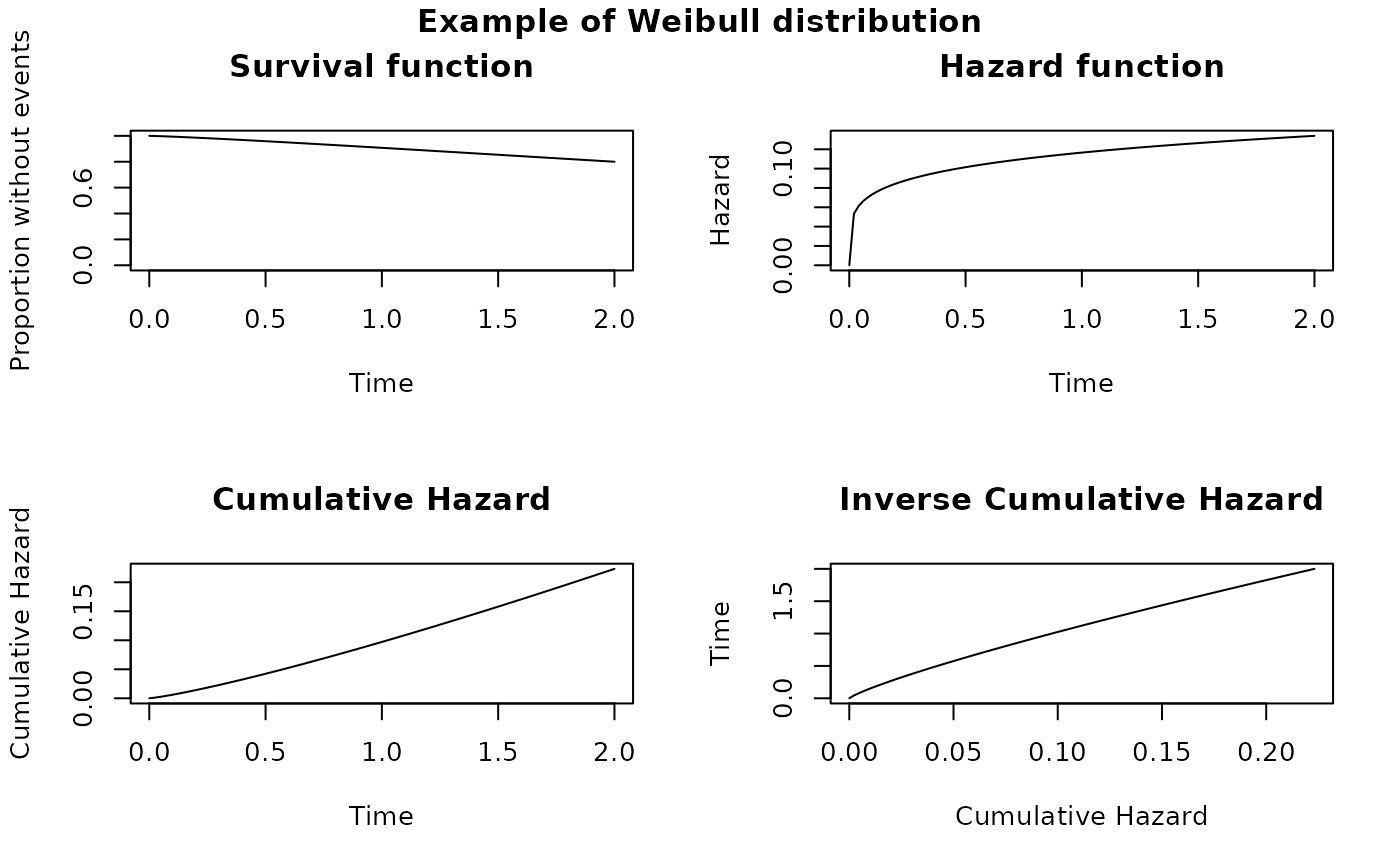
All the SURVIVAL objects have access to the functions described here
Usage
sfx(SURVIVAL, t)

hfx(SURVIVAL, t)

Cum_Hfx(SURVIVAL, t)

invCum_Hfx(SURVIVAL, H)

rsurv(SURVIVAL, n)

rsurvhr(SURVIVAL, hr)

rsurvaft(SURVIVAL, aft)

rsurveh(SURVIVAL, aft, hr)

plot_survival(SURVIVAL, timeto, main)

ggplot_survival_random(SURVIVAL, timeto, subjects, nsim, alpha = 0.1)

compare_survival(SURVIVAL1, SURVIVAL2, timeto, main)

ggplot_survival_hr(SURVIVAL, hr, timeto, subjects, nsim, alpha = 0.1)

ggplot_survival_aft(SURVIVAL, aft, timeto, subjects, nsim, alpha = 0.1)

ggplot_survival_eh(SURVIVAL, aft, hr, timeto, subjects, nsim, alpha = 0.1)
Arguments
- SURVIVAL
a SURVIVAL object
- t
Time
- H
cumulative hazard
- n
number of observations
- hr
hazard ratio
- aft
accelerated failure time
- timeto
plot the distribution up to timeto
- main
title of the graph
- subjects
number of subjects per group to simulate in each simulation
- nsim
number of simulations
- alpha
alpha value for the graph
- SURVIVAL1
a SURVIVAL object
- SURVIVAL2
a SURVIVAL object
Value
Depending on the function a proportion surviving, hazard, cumulative hazard, inverse of the cumulative hazard, a random draw or a plot
Details
rsurveh() generates random values under the Extended Hazards model of
Chen & Jewell (2001), which combines a proportional-hazards effect and an
accelerated-failure-time effect: h*(t) = hr * aft * h0(aft * t). It nests
the proportional hazards model (aft = 1) and the accelerated failure
time model (hr = 1) as special cases. Note this differs from the
Accelerated Hazards model of Chen & Wang (2000), h*(t) = h0(theta * t),
which is the special case hr = 1 / aft.
Functions
sfx(): Survival functionhfx(): Hazard functionCum_Hfx(): Cumulative Hazard functioninvCum_Hfx(): Inverse of the Cumulative Hazard functionrsurv(): Generate random values from the distributionrsurvhr(): Generate random values from the distribution under proportional hazard ratiosrsurvaft(): Generate random values from the distribution under accelerated failure time ratiosrsurveh(): Generate random values from the distribution under the Extended Hazards model (combined proportional hazards and accelerated failure time)plot_survival(): Plot of the survival functionsggplot_survival_random(): ggplot of the simulation of survival timescompare_survival(): Compare graphically two survival distributionsggplot_survival_hr(): ggplot of the simulation of survival times with hazard ratiosggplot_survival_aft(): ggplot of the simulation of survival times with accelerated failure timesggplot_survival_eh(): ggplot of the simulation of survival times with the Extended Hazards model
Examples
#' # Define a SURVIVAL object
obj <- s_factory(s_weibull, surv = 0.8, t = 2, shape = 1.2)

# Survival, Hazard and Cumulative hazard at time 0.4
sfx(SURVIVAL = obj, t= 0.4)
#> [1] 0.9681716
hfx(SURVIVAL = obj, t = 0.4)
#> [1] 0.09703794
Cum_Hfx(SURVIVAL = obj, t = 0.4)
#> [1] 0.03234598

# Time when the Cumulative hazard is 0.8
invCum_Hfx(SURVIVAL = obj, H = 0.8)
#> [1] 5.795862

# Draw one random survival time from the distribution
rsurv(SURVIVAL = obj, n = 1)
#> [1] 15.06117

# Draw one random survival time from the distribution under Proportional
# hazard, Accelerated failure time or the combined Extended Hazards model.
rsurvhr(SURVIVAL = obj, hr = 0.5)
#> [1] 2.994875
rsurvaft(SURVIVAL = obj, aft = 2)
#> [1] 1.989946
rsurveh(SURVIVAL = obj, aft = 2, hr = 0.5)
#> [1] 10.38445

# Plot the survival functions
plot_survival(SURVIVAL = obj, timeto = 2, main = "Example of Weibull distribution" )