Sample size with Uncertainty
John Aponte
2025-12-02
Source:vignettes/sample_size.Rmd
sample_size.RmdIntroduction
This example show in details how to construct a new factory of
DISTRIBUTION objects using a convolution of parameters to
propagate the uncertainty to the final calculation.
The estimation of sample size require the input of different parameters in a way that when the parameters are correct, the power to have a significant result is correct. However many times there are some uncertainty on the parameters and this is not reflected in the power.
The convdist package could help on explicitly express
uncertainty on those parameters and estimate the distribution of sample
sizes that would satisfy the power requirements of the assay.
We explore how to estimate the sample size for binomial outcome with
uncertainty and explain the details of how to construct a
DISTRIBUTION factory function.
Sample size for a proportion
For an individually randomized trial, the number of subjects per group could be defined as
In this formula, and are standard normal distribution values corresponding to upper tail probabilities of and respectively. This choice of sample size provides a power of 100(1 – )% to obtaining a significant difference ( on a two-sided test), assuming that the true (population) proportion in presence or absence of the interventions are and respectively
can be express on terms of as where is the relative risk.
In the real world, there could be uncertainty on the exact values of and as they may come from previous studies or surveys. What would be the distribution of if the uncertainty is taking into account?
A new DISTRIBUTION factory
We can construct a DISTRIBUTION object which would
produce random numbers taking into account the a probability
distribution for
and
See the code of new_UNIFORM function as an example of
how is a factory of DISTRIBUTION objects:
library(convdistr)
new_UNIFORM
#> function (p_min, p_max, p_dimnames = "rvar")
#> {
#>     stopifnot(p_min <= p_max)
#>     .oval = (p_max + p_min)/2
#>     names(.oval) <- p_dimnames
#>     structure(list(distribution = "UNIFORM", seed = sample(1:2^15,
#>         1), oval = .oval, rfunc = restrict_environment(function(n) {
#>         matrix(runif(n, p_min, p_max), ncol = 1, dimnames = list(1:n,
#>             p_dimnames))
#>     }, p_min = p_min, p_max = p_max, p_dimnames = p_dimnames)),
#>         class = c("UNIFORM", "DISTRIBUTION"))
#> }
#> <bytecode: 0x5579efb0cf48>
#> <environment: namespace:convdistr>
The function should return an structure which consist of a list of four named vector and a class attribute that should include “DISTRIBUTION” The components of the list are:
distribution : A character with the name of the distribution implemented. It is a good practice to use the same name also in the class attribute
seed : A numerical seed that is use to get a
repeatable sample in the summary function Use a
sample function to ensure each new object will have a
different seed
oval : The observed value. It is the value expected. It is used as a number for the mathematical operations of the distributions as if they were a simple scalar
rfunc(n) : A function that generate random numbers
from the distribution. Its only parameter n is the number
of drawns of the distribution. It returns a matrix with as many rows as
n, and as many columns as the dimensions of the
distributions, The rfunc should be defined within a
restrict_environment function to ensure only the variables
required to the function are included in the environment of the
function. This will prevent reference leaking which could make
the objects big and slow when saved in a file.
The factory of object for the sample size of proportions could be defined as:
#' Sample size for proportions, with uncertainty
#'
#' Create an new DISTRIBUTION object that produce
#' random drawns of the estimated sample size for
#' two proportions
#' @param p0 a DISTRIBUTION object that drawns for proportions in control group
#' @param logrr a DISTRIBUTION object that drawns log(RR) of the intervention
#' @param alpha significant value
#' @param beta  1-power
new_SAMPLE_SIZE <- function(p0,logrr, alpha= 0.05, beta=0.2){
  #checkings
  stopifnot(inherits(p0,"DISTRIBUTION"))
  stopifnot(inherits(logrr,"DISTRIBUTION"))
  stopifnot(0 < alpha & alpha < 1)
  stopifnot(0 < beta & beta < 1)

 # function of alpha and beta
  f_alpha_beta <- (qnorm(alpha/2,lower.tail = F) + qnorm(beta, lower.tail = F)) ^ 2

  # The expected value of the distribution with default name for the dimension
  # based on the oval value of the individual distributions
  v0 <- p0$oval
  v1 <- p0$oval*exp(logrr$oval)

  # expected value of the distribution
  .oval <- f_alpha_beta * (v0 * (1 - v0) + v1 * (1 - v1)) / (v0 - v1) ^ 2
  names(.oval) <- "rvar"

  #random function within a restricted environment where only
  #the specified variables can be accesed within the function
  .rfunc <- restrict_environment(
     function(n) {
       d_p0 = rfunc_p0(n)
       d_p1 = d_p0 * exp(rfunc_logrr(n))
       fab * (d_p0 * (1 - d_p0) + d_p1 * (1 - d_p1)) / (d_p0 - d_p1) ^ 2
     },
     rfunc_p0 = p0$rfunc,
     rfunc_logrr = logrr$rfunc,
     fab = f_alpha_beta
  )
  # Create the object with 4 slots
  structure(
    list(
      distribution = "SAMPLE_SIZE",
      seed = sample(1:2 ^ 15, 1),
      oval = .oval,
      rfunc = .rfunc
    ),
    class = c("SAMPLE_SIZE","DISTRIBUTION")
  )

}
Using the Sample Size object
As example, suppose that the incidence of anaemia in children under 5 have been estimated from a survey as 35% with 95%CI (30%,40%), and a prevention treatment that in other settings have shown to decrease anaemia by 50% with 95%CI(8% to 73%).
We can define a BETA distribution based on the CI as
d_p0 = new_BETA_lci(0.35,0.30,0.40)And a NORMAL distribution of the log(RR)
as
rr = log(1 - 50/100)
sd = (log((1 - 8 / 100)) - log((1 - 73 / 100))) / 4
d_logrr = new_NORMAL(rr,sd)
So the input distributions are
| distribution | varname | oval | nsample | mean_ | sd_ | lci_ | median_ | uci_ |
|---|---|---|---|---|---|---|---|---|
| BETA | rvar | 0.35 | 10000 | 0.35 | 0.03 | 0.30 | 0.35 | 0.40 |
| NORMAL | rvar | -0.69 | 10000 | -0.69 | 0.30 | -1.29 | -0.69 | -0.11 |
And base on this we can calculate the distribution of samples with those conditions
d_sample <- new_SAMPLE_SIZE(d_p0, d_logrr)| distribution | varname | oval | nsample | mean_ | sd_ | lci_ | median_ | uci_ |
|---|---|---|---|---|---|---|---|---|
| SAMPLE_SIZE | rvar | 95 | 10000 | 557654 | 49826919 | 37 | 96 | 2329 |

The oval value of the distribution give us the result we obtain from
the formula. With the conditions specified, a sample size of
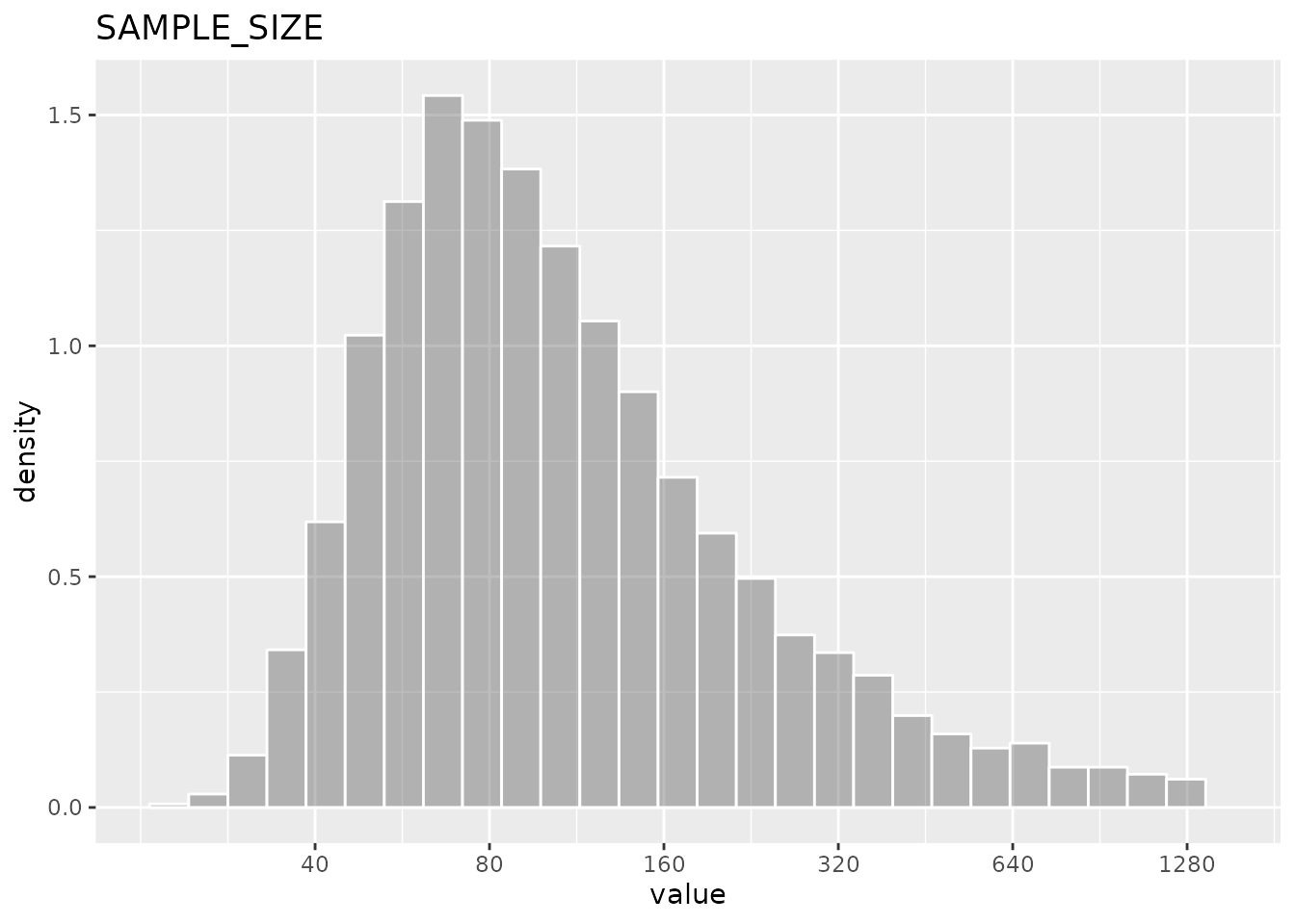
95 is required. However, the distribution is quite skewed
as you can see the mean and the median value are far, and the standard
deviation very big. This is because the sample size require for
combinations of low efficacy and low prevalence could be very large and
there is no restriction on how low could be the efficacy or the
prevalence, which although have low frequency, could happen in the
simulations.
rdrawn <- rfunc(d_sample, 10000)
f_ecdf <- ecdf(rdrawn)
n_80 = trunc(uniroot(function(x){f_ecdf(x) - 0.8}, interval = c(10,10000))$root)
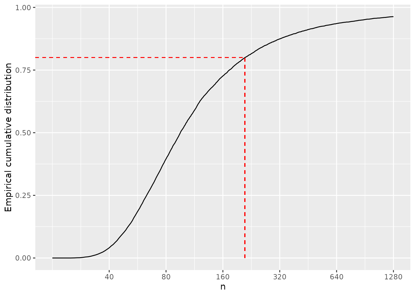
The empirical cumulative distribution values of a random sample of
the distribution show us that with 209 subjects per arm,
80% of the possible scenarios are covered

Enhance the Sample Size object
The function created above show us a distribution of sample size, but we can’t inspect condition on which a particular drawn is obtained, i.e. how low an prevalent anaemia value could be compensated with a high efficacy value? To do that we could create a second object that have drawns in several dimensions, the prevalence, the RR and the sample size so we can make a graph with the three values.
#' Sample size for proportions, with uncertainty (V2)
#'
#' Create an new DISTRIBUTION object that produce
#' random drawns of the estimated sample size for
#' two proportions as well as the samples from the parameters
#' @param p0 a DISTRIBUTION object that drawns for proportions in control group
#' @param logrr a DISTRIBUTION object that drawns log(RR) of the intervention
#' @param alpha significant value
#' @param beta  1-power
new_SAMPLE_SIZE2 <- function(p0,logrr, alpha= 0.05, beta=0.2){
  #checkings
  stopifnot(inherits(p0,"DISTRIBUTION"))
  stopifnot(inherits(logrr,"DISTRIBUTION"))
  stopifnot(0 < alpha & alpha < 1)
  stopifnot(0 < beta & beta < 1)

 # function of alpha and beta
  f_alpha_beta <- (qnorm(alpha/2,lower.tail = F) + qnorm(beta, lower.tail = F)) ^ 2

  # The expected value of the distribution with default name for the dimension
  # based on the oval value of the individual distributions
  v0 <- p0$oval
  v1 <- p0$oval*exp(logrr$oval)

  # expected value of the distribution
  ss <- f_alpha_beta * (v0 * (1 - v0) + v1 * (1 - v1)) / (v0 - v1) ^ 2
  .oval = c(p0$oval, exp(logrr$oval), ss)
  names(.oval) <- c('prevalence', 'rr', 'sample_size')

  #random function within a restricted environment where only
  #the specified variables can be accesed within the function
  .rfunc <- restrict_environment(
     function(n) {
       d_p0 = rfunc_p0(n)
       d_rr = exp(rfunc_logrr(n))
       d_p1 = d_p0 * d_rr
       d_ss = fab * (d_p0 * (1 - d_p0) + d_p1 * (1 - d_p1)) / (d_p0 - d_p1) ^ 2
       matrix(
         c(d_p0, d_rr, d_ss),
         ncol = 3,
         dimnames = list(1:n, c('prevalence','rr','sample_size')))
     },
     rfunc_p0 = p0$rfunc,
     rfunc_logrr = logrr$rfunc,
     fab = f_alpha_beta
  )
  # Create the object with 4 slots
  structure(
    list(
      distribution = "SAMPLE_SIZE2",
      seed = sample(1:2 ^ 15, 1),
      oval = .oval,
      rfunc = .rfunc
    ),
    class = c("SAMPLE_SIZE2","DISTRIBUTION")
  )

}
d_sample2 <- new_SAMPLE_SIZE2(d_p0, d_logrr)| distribution | varname | oval | nsample | mean_ | sd_ | lci_ | median_ | uci_ |
|---|---|---|---|---|---|---|---|---|
| SAMPLE_SIZE2 | prevalence | 0.35 | 10000 | 0.35 | 0.02 | 0.30 | 0.35 | 0.40 |
| SAMPLE_SIZE2 | rr | 0.50 | 10000 | 0.52 | 0.17 | 0.27 | 0.50 | 0.92 |
| SAMPLE_SIZE2 | sample_size | 95.31 | 10000 | 11495.32 | 620764.71 | 37.19 | 94.28 | 2765.09 |
ss <- rfunc(d_sample2, 10000)
df <- data.frame(ss)
df$category = cut(df$sample_size, c(0,150,Inf),include.lowest = T, ordered_result = T)
head(df)
#>   prevalence        rr sample_size  category
#> 1  0.3554726 0.5017183    93.97889   [0,150]
#> 2  0.4006951 0.5789086   115.32163   [0,150]
#> 3  0.3622292 1.1916518   775.78095 (150,Inf]
#> 4  0.3442364 0.5121539   103.24103   [0,150]
#> 5  0.3668436 0.6721487   226.83723 (150,Inf]
#> 6  0.3881253 0.3722672    47.74573   [0,150]
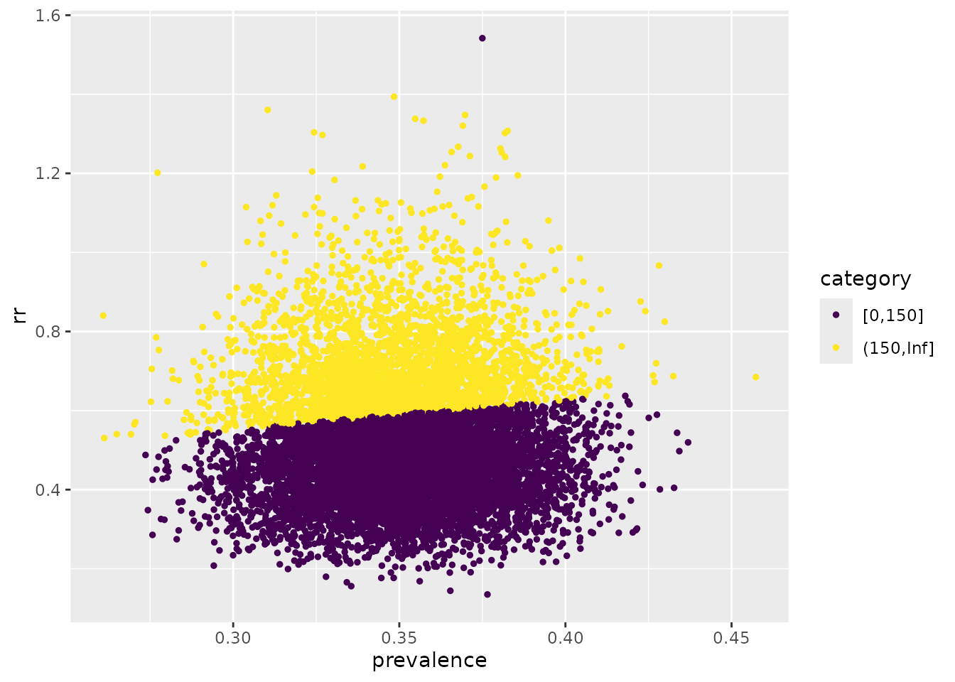
The following graph shows the combination of options that would lead to a sample size lower than 150 subjects

We see that under this particular set of conditions, it is possible to have more than 80% power in all prevalence range provided the relative risk is really lower than 50%.